

What is Diversification and How Does it Work?
One of the key concepts used by many successful investors is diversification. In this post, I’ll define diversification and explain how it works conceptually. I explain different ways you can diversify your investments and provide illustrations of its benefits in this post.
What is Diversification?
Diversification is the reduction of risk (defined in my post a couple of weeks ago) through investing in a larger number of financial instruments. It is based on the concept of the Law of Large Numbers in statistics. That “Law” says that the more times you observe the outcome of a random process, the closer the results are likely to exhibit their true properties.
Coin Flip Illustration
For example, if you flip a fair coin twice, there are four sets of possible results:

Estimating the True Probability of Heads
The true probability of getting heads is 50%. In two rows (i.e., two possible results), there is one heads and one tails. These two results correspond to the true probability of a 50% chance of getting heads. The other two possible results show that heads appears either 0% or 100% of the time.
If you repeatedly flip the coin 100 times, you will see heads between 40% and 60% of the time in 96% of the sets of 100 flips. Increasing the number of flips to 1,000 times per set, you will see heads between 46.8% and 53.2% of the time in 96% of the sets. Because the range from 40% to 60% with 100 flips is wider than the range of 46.8% to 53.2% with 1,000 flips, you can see that the range around the 50% true probability gets smaller as the number of flips increases. This narrowing of the range is the result of the Law of Large Numbers.
Following this example, the observed result from only one flip of the coin would not be diversified. That is, our estimate of the possible results from a coin flip would be dependent on only one observation – equivalent to having all of our eggs in one basket. By flipping the coin many times, we are adding diversification to our observations and narrowing the difference between the observed percentage of times we see heads as compared to the true probability (50%). Next week, I’ll apply this concept to investing where, instead of narrowing the range around the true probability, we will narrow the volatility of our portfolio by investing in more than one financial instrument.
What is Correlation?
As discussed below, the diversification benefit depends on how much correlation there is between the random variables (or financial instruments). Before I get to that, I’ll give you an introduction to correlation. Correlation is a measure of the extent to which two variables move proportionally in the same direction. It is important to understand that correlation does not necessarily imply causation, as illustrated by these examples.
In the coin toss example above, each flip was independent of every other flip. That is, there was no correlation.
0% Correlation
When variables are independent, we say they are uncorrelated or have 0% correlation. The graph below shows two variables that have 0% correlation.

In this graph, there is no pattern that relates the value on the x-axis (the horizontal one) with the value on the y-axis (the vertical one) that holds true across all the points.
100% Correlation
If two random variables always move proportionally and in the same direction, they are said to have +100% correlation. For example, two variables that are 100% correlated are the amount of interest you will earn in a savings account and the account balance. If they move proportionally but in the opposite direction, they have -100% correlation. Two variables that have -100% correlation are how much you spend at the mall and how much money you have left for savings or other purchases.
The two charts below show variables that have 100% and -100% correlation.


In these graphs, the points fall on a line because the y values are all proportional to the x values. With 100% correlation, the line goes up, whereas the line goes down with -100% correlation. In the 100% correlation graph, the x and y values are equal; in the -100% graph, the y values equal one minus the x values. 100% correlation exists with any constant proportion. For example, if all of the y values were all one half or twice the x values, there would still be 100% correlation.
50% Correlation
The graphs below give you a sense for what 50% and -50% correlation look like.

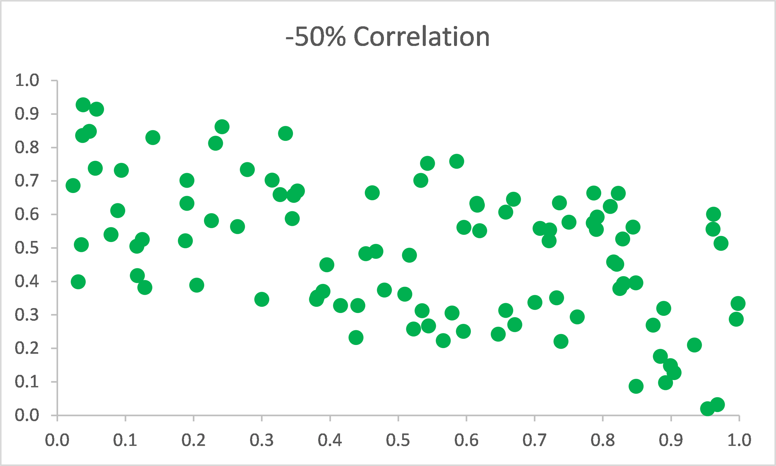
The points in these graphs don’t align as clearly as the points in the 100% and -100% graphs, but aren’t as randomly scattered as in the 0% graph. In the 50% correlation graph, the points generally fall in an upward band with no points in the lower right and upper left corners. Similarly, in the -50% correlation graph, the pattern of the points is generally downward, with no points in the upper right or lower left corners.
How Correlation Impacts Diversification
The amount of correlation between two random variables determines the amount of diversification benefit. The table below shows 10 possible outcomes of a random variable. All outcomes are equally likely.

The average of these observation is 50 and the standard deviation is 30. This standard deviation is measures the volatility with no diversification and will be used as a benchmark when this variable is combined with other variables.
+100% Correlation
If I have two random variables with exactly the same properties and they are 100% correlated, the outcomes would be:

Remember that 100% correlation means that the variables move proportionally in the same direction. If I take the average of the outcomes for Variable 1 and Variable 2 for each observation, I would get results that are the same as the original variable. As a result, the process defined by the average of Variable 1 and Variable 2 is the same as the original variable’s process. There is no reduction in the standard deviation (our measure of risk), so there is no diversification when variables have +100% correlation.
-100% Correlation
If I have a third random variable with the same properties but the correlation with Variable 1 is -100%, the outcomes and averages by observation would be:
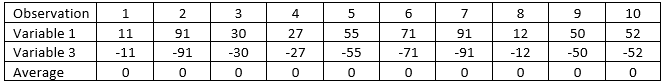
The average of the averages is 0 and so is the standard deviation! By taking two variables that have ‑100% correlation, all volatility has been eliminated.
0% Correlation
If I have a fourth random variable with the same properties but it is uncorrelated with Variable 1, the outcomes and averages by observation would be:
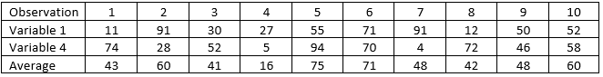
The average of the averages is 50 and the standard deviation is 17. By taking two variables that are uncorrelated, the standard deviation has been reduced from 30 to 17.
Other Correlations
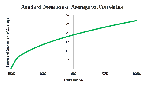
The standard deviation of the average of the two variables increases as the correlation increases. When the variables have between -100% and 0% correlation, the standard deviation will be between 0 and 17. If the correlation is between 0% and +100%, the standard deviation will be between 17 and 27. This relationship isn’t quite linear, but is close. The graph below shows how the standard deviation changes with correlation using random variables with these characteristics.
Key Take-Aways
Here are the key take-aways from this post.
Correlation measures the extent to which two random processes move proportionally and in the same direction. Positive values of correlation indicate that the processes move in the same direction; negative values, the opposite direction.
The lower the correlation between two variables, the greater the reduction in volatility and risk. At 100% correlation, there is no reduction in risk. At -100% correlation, all risk is eliminated.
Diversification is the reduction in volatility and risk generated by combining two or more variables that have less than 100% correlation.


